Hyperparameter Space


Going from molecular structure to mass spectra
Small molecules make most of our medicines, are the lingua franca of cell communication, metabolism, and signalling, and form an extremely diverse chemical landscape. And they’re everywhere in the environment. Even though we have millions of these little things cataloged in many databases, the chemical space of small molecules, even restricting to biological ones, remains relatively unexplored. It’s a brave ocean of uncharted waters full of potential therapies and materials. But, what do you do with a small molecule you just found? How can you characterize it and get an inkling of what it does? You can of course start putting it into living stuff and see how it behaves. Surely, however, we can at least get an idea of what it is and what it does before spending those hard-earned experimental dollars. Surely with all the data out there on small molecules we can use one of those fancy neural nets to predict their properties. How do we do this exactly though? Molecules, after all, are unlike just rows in a spreadsheet that you can spoon-feed to your tensor monster. As data types, they are information-rich and obey several types of regularities and symmetries: they exist as graphs of atoms with node and edge features as well as three-dimensional entities invariant to rototranslations with one or multiple conformations. Molecular graph relationships have also been encoded into semantic strings like SMILES, the ”language of (small) molecular structure”. Then there’s of course the hand-engineered, hard-won features of the ancestors. Bit vectors or “fingerprints” that have been traditionally used by computational methods since ancient times and are tried and true.
What representation then – graphs, 3D structures, fingerprints, or strings – is easiest to wield and which better unlocks the secrets of molecules? I wanted to get a sense of this by doing a property prediction exercise. However, I did not want to tackle just any property prediction toy problem, I wanted something that (1) might actually result in something useful and (2) was challenging enough to make me think about the different molecular representations in the context of the problem. I therefore chose a task that I had in the bucket list for some time: predicting mass spectra from (small molecule) molecular structure.
 The four paths of molecular machine learning
What is mass spec?
Mass spectrometry is a way of probing unknown molecules by basically blasting them into pieces. One takes an energy (ion) source and a way to isolate a stream of molecules and then blasts them. The bits and pieces (some of them might be fragments, or others the complete molecule) are energized (read ionized) by the blast and are then subjected to a magnetic field that sorts them by mass, giving a mass-to-charge readout which can be used as a proxy for mass. The resulting bits and pieces provide a signature, sort of a hash, of your molecule. Though blasting stuff is fun in general, the appeal of mass spectrometry actually comes from its high-throughput: you can read thousands if not tens of thousands of unique molecules per experiment in any relatively complex sample.
 Mass spectrometry is taking an ion source, blasting a molecule, then reading out the ions and fragments sorted by a magnetic field. Above is a depiction of totally how this works in detail
The hash of the molecule though (i.e. its mass spectra), is typically imperfect. Many molecules have the same mass for example, and when you have a complex mixture of stuff, it’s hard to know which bits and pieces correspond to which molecules. However, you can get pretty creative with mass spectrometry. One common technique is to put two mass spectrometers in tandem, you then blast the molecule with the first one, then measure, then isolate a mass of interest, then blast and measure again. This is known as MS2 mass spectrometry and it increases the “resolution” of your hash. MS2 is typically used for compound identification, by comparing the mass spectra of a molecule with other mass spectra of other molecules previously measured. You can actually keep adding tandems of spectrometer readouts fragmenting the fragments recursively for n steps, producing what’s called MSn readouts. As you can imagine MSn readouts increase your “hash resolution” but unfortunately the mass spectrometers capable of such protocols are expensive and not widely used. Thus, when analyzing mass spectra for molecular identification, one usually looks at MS2 data.
Mass spec is a very flexible technique and can be coupled with wild things like particle accelerators and do cool stuff like spatially resolve molecular signatures, but I won’t go into MS hype because this post would be like 10x more long.
 A freaking particle accelerator plugged into a mass spectrometer. BTW this is how radiocarbon dating is done apparently.
Why mass spec?
There are two main reasons I wanted to try my hand at this: speed and open data. As you can imagine, there are several tools that already predict spectra (specifically MS2 spectra) from molecules, most of them used for compound identification. They vary in strategy but the state of the art uses quantum mechanical calculations and molecular dynamic simulations. This is a very costly calculation that can take up to an hour or more per molecule. A speedier approach uses hand fragmentation rules as well as a cool probabilistic model for simulating fragmentation from types of bonds and molecular structure, but still takes up to minutes depending on the size of the molecule. Why is speed important? A fast method would allow the generation of 100s of thousands or even millions of spectra for known molecules, boosting compound identification considerably. So one question is: can we sacrifice detail in the spectra in exchange for speed?
The second reason is open data. There is actually one deep learning based method that was explored by google brain a few years back that is pretty fast but it only works on electron impact ionization (EI) mass spec, which is a fancy way of saying that it can only look at molecules in the gas phase. Unfortunately, life mostly happens in the liquid phase (which in mass spectrometry is probed via blasting methods called electrospray ionization, or ESI) so this limits its application in bio. One of the reasons that it was trained only on EI mass spec is that, at the time, there just weren’t many good ESI datasets pairing molecular structures with mass spectra and NIST had been maintaining a good curated EI set with around a hundred thousand measurements. Fortunately, these past couple of years there has been a growth spurt of a few open databases with ESI data, including the awesome GNPS platform, that have gone from a few thousand measurements to several hundred thousands. The data might be noisier and needs to be more curated than e.g. the NIST data, but it is totally open, no-strings-attached (the NIST data itself needs to be bought for some thousands of dollars). It means that data is available to play with a few models and hey, if I can extract any win for open databases, then it’s an overall win in my book.
There is actually a third reason – I recently bought a gaming laptop for FFXIV raid nights and finally have a dedicated GPU to play with for my side projects. Gaming and science go hand-in-hand after all.
Problem definition
Ok, enough motivation, what do we actually need to do here? GNPS has on the order of 600k+ of molecule/mass spectra pairs: the molecules being presented as SMILES strings and the mass spectra as two lists, one with the M/Zs and one with their respective intensities.
 A sample molecule and it’s MS2 spectra (M+Na adduct – we’ll define this in a second)
We’ll filter this a bit before proceeding, both to make things easier on the models and training (I only got a laptop to train after all).and for other technical reasons:
- We’ll only take ESI data, like we mentioned earlier
- We’ll focus on molecules having at least 10 spectral peaks, meaning that there’s actually something a bit complex to predict
- We’ll only consider molecules with spectral peaks with a mass-to-charge M/Z ratio of at most 2000. Anything with a mass larger than that is not that small of a molecule.
- We’ll only train on positive ionization mode data. In mass spec, when we blast the molecule, we can either do it with positive or negative charge ions. For, errr, reasons, positive mode data turns out to be a bit more informative and is generally more abundant.
- We’ll only train on molecular structures that are (1) valid in a sense that their SMILE strings can be parsed and (2) we can quickly obtain a 3D representation of them by passing them through a simple 3D geometry optimizer (more info on this below). This will be necessary for one of the models – the 3D one – that we’ll consider.
We’ll also only focus on molecules with ion types that are somewhat abundant in the GNPS data. Not terribly important (although yes terribly important, but not for defining the problem at least), molecules tend to carry some ions when you blast em (most commonly, if you’re giving it a protein charge, it will carry a mass of a proton, but you also see flavors carrying e.g. nitrogens and other weird stuff like a double positive charge or a water molecule attached). These adducts are typically written as M+A where A is the atom or species being carried along. I ended up taking the ions that had at least 10k examples, which were M+H, M+Na, M+NH4, M-H2O+H, and somewhat rarely M-H.
All in all, these filters winnow the dataset down to 130k+ measurements, which is just shy from the 150k that the google brain study used to train their net.
Spectra representation and pre-processing
Mass spectra are interesting objects: they are sets of pairs of mass-to-charge values and their intensities. Mass-to-charge values can be important up to the 2nd to 3rd decimal value. One naive approach I tried at first is having one net predict the mass-to-charge values as a continuous regression task from the molecule, then using the predicted values plus the molecule to again to predict the intensities (also as continuous regression targets). The question becomes how to actually set up the continuous regression M/Zs, do you put them randomly into a vector? Sorted? How do you treat spectra of different lengths? Do you treat the whole prediction as a set (in which case you have to do some stuff to do some tricks to make it permutation invariant)? I tried a few of these things but they didn’t quite work and the net had trouble predicting the M/Zs, consistently low balling them. Instead, I fell back to the courser-grained representation used by google brain in their paper: M/Z are rounded to the nearest integer, which becomes the index in a vector of intensities (if two M/Zs round to the same integer, I take the max intensity).. So if we have a limit of 2000 M/Z for our spectra, we’re going to predict a 2000 dimensional vector of intensities.
Anyone familiar with mass spec might be shaking their heads right now. There is a lot of information that is potentially lost when you round an M/Z to the nearest integer (remember, many things map to the same mass – if you round stuff, many more will have this “hash collision” failure). Losing all decimal points of precision seems like too much, so I settled on a compromise: I would also predict the decimal expansion of the max intensity M/Z for each M/Z integer bin. That way, we end up with a 2000 X 2 = 4000 dimensional vector, the first half would have the intensities and the second half the decimal expansion of the most intense M/Z. This gives us an additional boon, we can see how precise the spectral representation is according to our net.
The intensity values themselves can vary a bit by instrument and since this is open data you might have a lot of heterogeneity there (some reading on the 100s others on the 10s of 1000s). Thus, I’m predicting relative intensities, that is, set as a fraction of the maximum intensity in the spectra. Interestingly, this helped but was not as super crucial as I thought. Finally, both intensities and decimal expansions are log-transformed (base ten) with a plus one pseudo-count to avoid -inf in the cases where e.g. an intensity is zero.
Covariates
Before I describe the models and molecular representations I tried, there’s a couple of things that we need to include as covariates that affect the measured spectra. The first is the ion type which we already mentioned above, which we include one-hot encoded as an input to the models. The second is the energy used by the ion source, which basically measures how intensely we’re blasting the molecule. As you can imagine, the amount of fragments and their spectral peaks depend on how strong the ion source is. But although the energy is many times recorded in the metadata, different instruments/protocols/labs might give different results even with the same energy. So instead of relying on metadata, I tried do an unsupervised assessment of the level of fragmentation of a spectra by looking at the intensity of the mass peak corresponding to the mass of the molecule (the precursor in mass spec parlance) relative to the sum of the total spectra (in practice I look not only at the precursor mass intensity but also plus minus some M/Z window which both takes care of the mass shift from ions attached to the molecule – i.e. the ion type – and other weirdness that sometimes occurs). I log-transform these values and call them fragmentation levels. Interestingly, fragmentation levels follow a somewhat bimodal distribution, corresponding to low and high energy settings. I input fragmentation levels into the model as a one-hot encoding, choosing from an integer rounding of the most common fragmentation levels, from -4 to 0.
 Histogram of fragmentation levels (log-transformed ratio of precursor mass intensity vs total intensity)
Models and molecule representations
As mentioned above, the whole point of this exercise was to get a sense of the four ways you can achieve molecular machine learning. These are the model contenders.
Fingerprint MLP
First up we’ll try to use molecular fingerprints. Particularly, we’ll use the flavor everyone likes: the extended connectivity fingerprint (ECFP) which encodes the identity and connectivity pattern of each atom using the Morgan algorithm. ECFPs are pretty effective across the board and they capture local and distant connectivity patterns in an iterative fashion. For a super friendly introduction, check out this page. We’ll use a 1024 bit fingerprint, meaning a 1024 vector of zeros and ones for the molecular representation. We’ll then feed this into a simple, deep multi-layer perceptron (MLP). These days, it seems that MLPs are synonymous with MLPs with residual connections, so each layer of the MLP will actually be a residual block. I used SiLUs for the activating function, which gave a slightly better performance than ReLUs but not by much. The architecture is super straightforward:
 Molecular fingerprint-based MLP architecture
GCN
Then, I tried a graph convolutional neural network using the awesome torch_geometric package. Graph convnets (GCNs), or more generally message passing networks, come in many many many flavors now and I was quite overwhelmed by the number of choices:
 This is just like a third of the convolution layers available…also there’s a similar list for pooling
I decided to take the vanilla GCNs – the real OGs. In any case, all of these modules basically take graphs as inputs, which means a list of edges and a set of features for each node and each edge. What features do we include for nodes and edges? Here, things start to get a lot less standardized than in the fingerprint world and you really have to get the know-how directly from the practitioners. After scrolling through kaggle notebooks and the deepchem source, I settled on using a set of properties that were easily extracted from each atom and bond using RDKit and put them as node and edge features respectively. Deciding how many atom properties and how to encode them into node features was probably the thing that required the most trial and error and made a huge impact on performance. I first started with a few basic properties and performance was pretty low, but then added quite a bit more and it started to get a bit better. What was interesting is that how I encoded the atom properties mattered a lot as well. For example, encoding the valence and number of hydrogens in a one-hot fashion (like the deepchem folks) instead of directly as numbers really helped.
What was the final architecture here? It basically consisted of a sequence of GCN layers and then a global max pooling at the end (I also tried sum and mean as well as more fancy methods like jumping knowledge but they gave similar results). The pooled features are then appended to the graph-level covariates (ion type and fragmentation level) and are then fed to a linear layer with residual connections and then a layer on top to convert to spectra feature space.
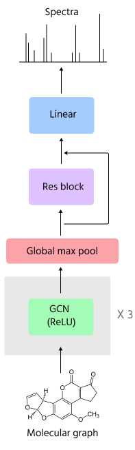
Graph convolution architecture
EGNN
Let’s get a bit more fancy and use an E(3) equivariant graph neural network (EGNNs). EGNNs are GNNs that not only have graph connectivity and node and edge features, but also a 3D position for each node and ensure that the layer transformation functions are equivariant to rotations, translations, and reflections of these 3D points (this is called the E(3) group). I used the Garcia Satorras implementation, which is a very simple addition of cross node position distances to the edge operation of the graph convolution that turns out to be E(3) equivariant.
The GNPS data doesn’t actually have 3D positions computed for each molecule, so I used the very simple MMFF forecefield in RDKIT to compute them from scratch. As with the GCNs, we also add a max global pooling operation and a residual linear head to include the ion type and fragmentation level covariates to then output a spectra.

Eqivariant graph neural network (EGNN) architecture
SMILES transformer
Finally, why not try the NLP route and use a string representation of molecules? The most popular is the ubiquitous SMILES, the very same format that the molecules in our dataset are in. SMILES are encoded using a similar algorithm to the ECFP fingerprints, but instead of saving the connectivity as bits, it has a language of its own. To go full NLP, we’ll be actually finetuning a masked language model that has been already trained on a medium size corpus of molecular SMILES. Specifically, we’ll be using the ChemBERTa model trained on the ZINC database. Getting the model to spit out vectors from SMILES is pretty easy since it uses the Huggingface API. Initially, I don’t know why I tried to code up a model that held the whole ChemBERTa model with frozen parameters as the initial layer and a simple head on top. This of course consumed most of my GPU memory and was super unwieldy to train. I guess I thought I could get fancy by unfreezing some layers but it never worked out. In the end, I stuck with just vectorizing the SMILES first using the pretrained ChemBERTa and then just training an MLP identical to the fingerprint one using those representations.
 ChemBERTa-based MLP architecture
Loss, training, and evaluation
The loss function here is pretty straightforward. Nothing more than the mean squared error. I tried mean absolute error as well but in general it gave weirder looking spectra. For the optimizer, I used Adam with the magic learning rate 3e-4. I half-heartedly tried using some learning rate schedulers and AdamW but they actually performed worse, likely because they need to be optimized further and I just was running out of motivation at that point. For hyperparameter scans, these are the values that I scanned per model (the ranges were short enough that I just scanned them all):
| Model | Hidden units | Layers | Batch size |
|---|---|---|---|
| mlp | 512,1024,2048 | 1-7 | 16,32,…,256 |
| gcn | 512,1024,2048 | 1-4 | 16,32,…,128 |
| egnn | 512,1024,2048 | 1-4 | 16,32,…,128 |
| bert | 512,1024,2048 | 1-7 | 16,32,…,256 |
After the hyperparameter scan, I chose the best parameters for a final “production” run that I trained for a little longer, 100-200 epochs depending on the model. One interesting tidbit is that the graph convolution (GCN and EGNN) models had to be shallowish, because adding more layers led to some wild learning curves full of beautiful NaNs. After digging around a bit, it looks like it’s known that these architecture suffer from vanishing and exploding gradient issues. There are some architecture tricks that are advertised to address these issues, but I didn’t try them..
For training splits, I had a training set for training plus a held out test set for monitoring test loss (an 80/20 split) and a completely separate validation set (of ~4k molecules) that I used to inspect more deeply how the models did in the end. I didn’t go out of my way to eliminate very similar molecules in train, test, and validation sets, I figured that if I reduced the dataset further, I would have been left with too little data, especially considering the fragmentation levels and ion type covariates. Multiple measurements on the same molecules could also give the network a sense of uncertainty these spectra carry…probably.
For evaluation, other than test loss, I assessed the intensity and the M/Z decimal expansion part of the predictions separately. For the first, I measured performance using an M/Z weighted cosine similarity, which is what many methods in this field use. For the second, I measured the accuracy of the predicted M/Z as a mass percentage of the true one (difference of prediction and truth, divided by truth).
Results
So how did it turn out? Let’s take a look at the test/validation loss as well as average cosine similarity and ppm in the validation set:
| Model | Test error | Validation M/Z percent error | Validation cosine similarity |
|---|---|---|---|
| mlp | 1.87e-4 | 0.052 | 0.39 |
| bert | 1.79e-4 | 0.054 | 0.35 |
| egnn | 1.87e-4 | 0.057 | 0.30 |
| gcn | 1.88e-4 | 0.057 | 0.28 |
Interestingly, the deeper MLPs based on fingerprints and SMILES do the best. Interestingly, the EGNN comes on top on test loss, but the MLPs win on cosine similarity by some margin. As you can see, the EGNN does add something useful compared to the vanilla GCN, which is pretty cool. I looked at the top/bottom 10 best/worst predictions for each model. All of them nailed simple molecules that are super common, like nucleotides (I wonder if that’s a training set contamination) with decent fragmentation levels. Interestingly, the ones where all models did worse was overpredicting spectral fragment peaks for molecules that had low fragmentation level and thus did not have complex spectra. I think this highlights why learning spectra from molecules is a difficult problem: sometimes a molecule fragments and sometimes it doesn’t even in the same-ish conditions, the spectra can and does change with all these variables.
 A couple of examples of the best and worst predictions of the MLP fingerprint model
I wanted to compare head to head to other methods but 4k molecules would take a looong time to run on spectral simulators that use quantum calculations. Instead, I have a CFMID4 run queued up (in my laptop, remember I still do gaming) and will update and report back with more numbers. The CFMID4 paper generally has 0.3ish average dice similarity in their results, which is sort of like cosine similarity? Anyway, I’ll have to wait and see.
Closing thoughts in the form of questions
Are the models available for use?
Yes! I made a package that you can install locally and run, hopefully easily (you do have to install torch_geometric first though, which depends on your pytorch and gpu configuration).. The goal was to have a runnable program that could get to MS2 spectra from just SMILES. I’ve also made a simple colab that’s easy to run.
Do you have the processed data somewhere?
Yeah, I made a zenodo entry with the processed GNPS data as well as the 3D geometries in SDF,. though in hindsight this might not have been a good use of zenodo….
Is this the best you can do?
Hopefully I gave the impression that I cut some corners to get to the end, which means that there’s likely a lot more that you can do with the data. For starters, I don’t think I’m even close to the “state-of-the-art” of even this dataset. For example, it turns out that the EGNN was generally harder to train, and I had to tweak the learning rate a bit (to 1e-4 in the end). However, I don’t think I saturated its learning capacity (as opposed to the fingerprint MLP, which really hit a plateau) and I can easily see how its performance could be made better by just training for longer. For the ChemBERTa SMILES MLP, I only used the most basic ZINC trained model – their pubmed model should have learned better representations. There are also still a lot of tried-and-true things you can do to squeeze more performance, like stochastic weight averaging and actually scanning learning rates and learning schedules properly.
What’s the best way to improve performance?
By far the best way to improve would be to convince mass spec folks to deposit MOAR DATA to GNPS. I cannot stress enough how important open databases are, especially in fields like mass spectrometry where they have historically been closed and behind proprietary software. Hopefully this adds to the evidence of how powerful being aggressively open is. On that note, my hypothesis is that enough MSn (n>=2) spectral data (e.g. millions of spectra) would get a transformatively accurate compound identification model. Just imagine all the chemical diversity out there hidden right under our noses.
Did you learn anything on the machine learning side?
I think so! Aside from technical stuff, I think we really should have self-supervised, pre-trained models like ChemBERTa but for all modalities, including 3D equivariant ones. Training these things from scratch is a bit onerous and is limited by the practitioner’s GPU setup. There’s already work on pretraining graph neural nets that goes back to 2019, we just need to make pretrained models more popular and adapt them to the equivariant setting.
Acknowledgements
Thanks to the awesome Ming Wang for pointing me to the GNPS database and discussions – and to all of the contributors to GNPS, you rock.