Hyperparameter Space


A Hacker’s Guide to Equivariance
Geometric deep learning is a field that has picked up considerable momentum recently. And with good reason, as it deals with ways on how to reason over objects (like graphs, meshes, and protein structures) that are tied to impactful tasks downstream (like predicting molecular properties and automating animation). Additionally, it’s setting up a framework that tries to retroactively explain many of the successes of deep learning with the hope of extrapolating lessons learned to new, more challenging domains. In this post, I’ll give a brief intro to the main concepts behind geometric deep learning and demonstrate how to code a simple module that implements one of the basic geometric deep learning tenets – equivariance for any symmetry – from scratch.
What is geometric deep learning?
Geometry can mean many things to different people: it might conjure images of manifolds in some minds, topological and distance properties, or particular arrangements of graphs in others. The “geometric” part in geometric deep learning, however, deals with the most abstract part of geometry: symmetries. Symmetries are composable functions under which an object can be transformed and remain unchanged, i.e., the objects are invariant to such transformations. The nature of the object and how to reason over its properties are tied to the symmetries that apply to it. They establish the rules by which we define geometric spaces. For example, objects in the Euclidean space are invariant under rotation and translation symmetries (a 3D object is the same object no matter how you turn it and move it around), while arbitrary topologies are defined by continuous scaling and deformation symmetries (where a teacup and a doughnut are considered the same thing). As a consequence, specifying what symmetries apply to an object allows automated algorithms to reason over complex and rich structures while respecting their nature, enabling machine learning methods over modalities like grids (e.g. images), graphs (molecules, social networks), and manifolds (e.g. meshes).
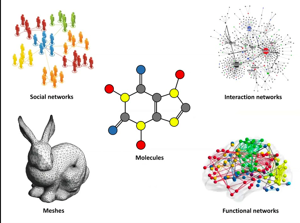 Geometric deep learning tries to inject symmetries into machine learning models to make it more natural to reason over complex objects like graphs and meshes. Taken from “Geometric Deep Learning Grids, Groups, Graphs, Geodesics, and Gauges” by Bronstein et al.
Formally, symmetries are defined as mathematical groups: a set of objects and an operation (in this case, composition) with a neutral element and inverses for each object. Like vector spaces and the like, groups have a “basis” set of generators from which you can generate the entire group. These groups act on vector spaces by applying the functions represented by each object. The group of rotations therefore acts on 3D objects by, well, rotating them. If the action of the group is linear, we can choose matrices as actions themselves. These matrices are called representations – for the rotation case, we can simply choose the rotation matrices as our representation. Note that these groups need not be finite and can have even more structure to them like Lie algebras.
How do we inject such symmetry constraints into machine learning models? Let’s take neural networks for example, which are compositions of functions in high dimensional spaces. Each intermediate transformation in the composition chain can be perhaps conceptualized as a metaphor in which the machine is manipulating the input object, examining it from different angles and giving intermediate assessments, then collate those assessments to give the final verdict. We want the assessments and the verdicts to be invariant in the way the symmetries of the objects dictate (an apple is still an apple if it’s rotated or not). But we also want the manipulation of the object to be consistent with our symmetries: whatever our machine is thinking when looking at the object it should shift in the same manner as our symmetries dictate. This last constraint is known as equivariance and it’s the other piece of the puzzle on how to introduce symmetries into the model. Equivariance to a function $f$ given a symmetry $g$ is simply saying that application of both things are commutative, e.g. $f(g(v)) = g(f(v))$, where $v$ is in the vector space.
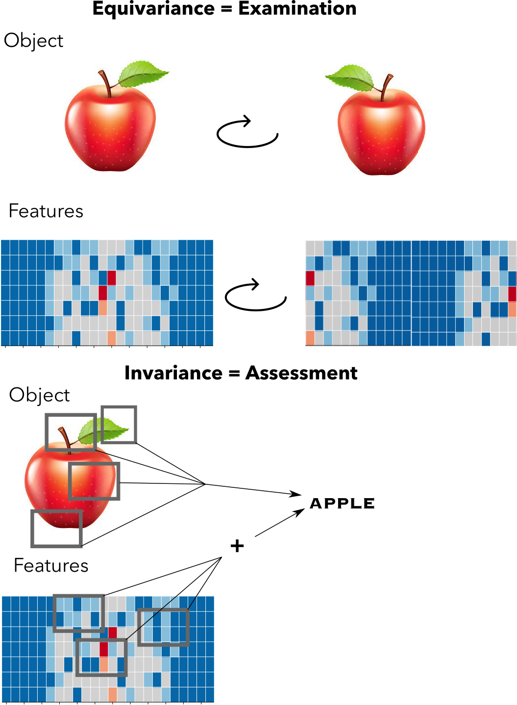 Equivariance is like examining an object: it’s features transform in accordance to an objects symmetry actions. Invariance is more like assessing an object, aggregating all of its features in some way to give a set of veredicts
Equivariance is actually the property that motivated geometric deep learning in the first place. Indeed, part of the success of convolutional neural networks was attributed to their property of being translationally equivariant. Even in parts of networks where equivariance was not baked in, it has been observed that it arises naturally in some contexts. Pulling the convolutional thread, Cohen and Welling generalized CNNs to be equivariant to any group, a strategy that Cohen later expanded into a full theory, setting convolution as the centerpiece of equivariance network design. This work has been expanded to transformers in some groups like roto-translations and others, as well as very general design algorithms for equivariant MLPs. The theory also seems to apply retrospectively to popular architectures – e.g. a slightly modified versions of LSTMs are time-warping equivariant – which has led to the authors laying out a manifesto of sorts for categorizing network architectures and the spaces/objects they operate: a geometric deep learning blueprint for understanding and designing equivariant architectures.
But what does equivariance actually buy you? Designing these architectures is not trivial and implementations can get really slow. The main advantage that has been observed is sample efficiency: equivariant networks tend to work in smaller data regimes. Particularly, data augmentation schemes are redundant in equivariant networks as there is no need to teach the network that translated/rotated versions of an object are the same since it’s already baked into the architecture. In a way, the amount of true symmetry equivariances and invariances a model has is a dial of how much data it needs: in one extreme a completely naive network will need a lot of data to learn about all the symmetries and in the other extreme it might resemble a natural law where no data is required as the symmetries are almost all known.
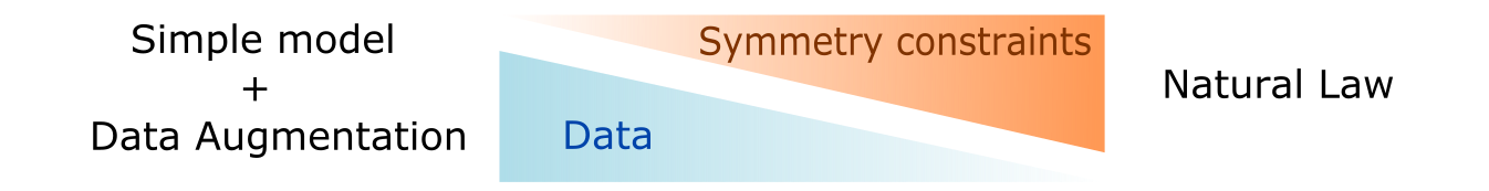 Symmetry constraints and data augmentation are two sides of a coin: with more symmetry constraints, less data is required approximating a natural law
Hacking our way towards equivariance
Note: all of the following code is available in a colab notebook
Doing is learning! What if we try to implement a deep learning module that is equivariant to some symmetry from scratch? Let’s consider a toy problem in computational biology: predicting the binding energy of some fixed transcription factor to various DNA sequences. In this problem, you have a DNA sequence (made up of TGCAs) and you want a regressor to predict a binding energy to a fixed transcription factor. For example, the TATA-box binding protein is a transcription factor that binds sequences that have a TATA-box sequence motif and the binding energy varies depending on how similar to the motif a part of the DNA sequence is. DNA sequences can come from many organisms and evolve in different ways, so you expect the sequences you will examine to be mutated versions of each other, so e.g. ATTGCAAA might have the same biological meaning as a slightly mutated version of it, say ATTTCAAC. This way, you can sort of visualize that the way a functional sequence motif “moves” across evolutionary time is through mutations – there is a sort of “mutation” symmetry that the sequences follow.
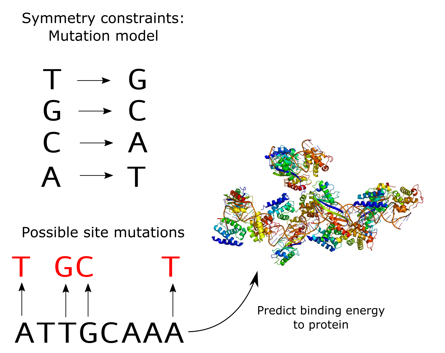 Setup of our problem for predicting binding energies of various DNA sequences to a particular protein. Symmetries here are defined by point mutations of the DNA sequence
How do we set this up? There are two main objects we must deal with here: DNA sequences and the symmetries themselves. DNA sequences will be fed into our network using the standard one-hot encoding per nucleotide, laid out as four-dimensional binary vectors (one dimension for each nucleotide) concatenated together to form a sequence. Thus, sequences will be our vector space, which we’ll setup as a parent class. We’ll then have a Sequence class inheriting from it that will put together vectors in the context of sequences, with some auxiliary methods to go from/to nucleotide strings:
class VectorSpace:
 DIM = None

 def __init__(self, vec):
   self.vec = vec

 @staticmethod
 def sample(n_samples):
   return NotImplemented


NUCLEOTIDES = 'TGCA'
# Toy example, we’ll just consider sequences of length 10
SEQ_LEN = 10
class Sequence(VectorSpace):
 DIM = SEQ_LEN * 4
 OH_VECS = {
     'T': np.array([1, 0, 0, 0]),
     'G': np.array([0, 1, 0, 0]),
     'C': np.array([0, 0, 1, 0]),
     'A': np.array([0, 0, 0, 1]),
 }

 IDX_TO_VEC = {
     np.argmax(v): k
     for k, v in OH_VECS.items()
 }

 def __init__(self, vec):
   super(Sequence, self).__init__(vec)

 @staticmethod
 def from_str(seq):
   return Sequence(vec=np.hstack([Sequence.OH_VECS[s] for s in seq]))
  def to_nuc(self, vec):
   return Sequence.IDX_TO_VEC[np.argmax(vec)]

 @property
 def seq(self):
   return ''.join(
       [
        self.to_nuc(self.vec[i:i+len(NUCLEOTIDES)])
        for i in range(0, len(self.vec), len(NUCLEOTIDES))
       ]
   )

  @staticmethod
 def sample(n_samples):
   return [Sequence.from_str(''.join(np.random.choice(list(NUCLEOTIDES), size=SEQ_LEN))) for _ in range(n_samples)]

 def __repr__(self):
   return self.seq
Thus, you create sequences with Sequence(a_vector) and you can use the utility methods to get the string representation. Next, let’s create a class for symmetries, which we’ll name Sy here. To make things simple, we will ask for the symmetry to be instantiated with a dictionary of generators, which will map strings to functions (we are assuming that our symmetry generators are finite). The functions themselves will be used as the actions of the group on an element of a vector space. We act on a vector by naming the generators used and composing the functions in that order:
class Sy:
 def __init__(self , generators):
   self.generators = generators

  def act(self, X, *names):
   composition = functools.reduce(
       lambda f, g: lambda x: f(g(x)),
       [self.generators[name] for name in names],
       lambda x: x)
   return composition(X)
Ok! Now let’s build our mutation symmetry group. First of all, we’ll have to declare what nucleotide is likely to mutate to which other – Ts might mutate to Gs more often Gs to Cs, etc. To make things super simple, we will say that T will always mutate to G, G to C, C to A, and A to T. Remember that we can mutate a nucleotide per position, so we’ll need SEQ_LEN generators times four, one for each transition in one position:
def generate_mutate_fun(position):
 def mut_fun(seq):
   mut_vec = seq.vec.copy()
   pos_slice = slice(position * len(NUCLEOTIDES), len(NUCLEOTIDES) * (position + 1))
   # the following shifts the one hot encoded bit cyclically to the right
   # so the mutation model is T -> G, G -> C, C -> A, A -> T.
   mut_vec[pos_slice] = np.roll(seq.vec[pos_slice], 1, axis=0)
   return Sequence(mut_vec)
 return mut_fun

mutation_generators ={
       f'mut{pos}': generate_mutate_fun(pos)
       for pos in range(SEQ_LEN)
}

# Add identity
mutation_generators.update({'id': lambda x: x})

# Build mutation transformation group
mutate = Sy(generators=mutation_generators)

# Example acting on a sequence
seq = Sequence.from_str('CCCCTATTAC')
mutate.act(seq, 'mut0', 'mut0', 'id', 'mut5') # output is TCCCTTTTAC
The reason I wrote the generator functions in such a weird way (shifting the nucleotide vector) is mostly for illustrative purposes that will be clear below, but I could have written it plainly as substituting the subvector/character at the appropriate position. It’s important to emphasize that I want the API to look as functional and general as possible – we’ll worry about the mathematics to make it rigorous later.
Equivariant versions of a function
There are several ways we can go about and design an equivariant module. Here, I will take the route of having an arbitrary learnable function – representing our deep learning module – and getting a version of it that is actually equivariant to our symmetry. Specifically, given a function $f$ and our symmetry $g$, what we want is a function $f_{equiv}$ that will remain as faithful as possible to $f$ but that is also equivariant, i.e. $f_{equiv}(g(s)) = g(f_{equiv}(s))$. In other words, we want to solve for an optimization problem that looks like this:
\begin{equation*} argmin_{f_{equiv}} ||f(s) - f_{equiv}(s)||^2_2 \end{equation*} \begin{equation*} f_{equiv}(g(s)) = g(f_{equiv}(s)) \quad \forall v \forall g \end{equation*}
Here I’m using an $l2$ norm as a loss function to minimize to illustrate. To simplify things even further, let’s say $f$ is linear so that $f(s)=Ms$. In which case the optimization problem becomes: \begin{equation*} argmin_{M_{equiv}} ||Ms - M_{equiv}s||^2_2 \end{equation*} \begin{equation*} M_{equiv}g(s) = g(M_{equiv}s) \quad \forall s \forall g \end{equation*}
Let’s reaaaaaaally simplify this and say we want this to hold for some finite set $s \in S$ by either sampling the vector space or looking at its basis, and focusing just on the generators of the group $g \in G$. In that case, we can plug in the equivariance constraints as Lagrangian multipliers:
\begin{equation*} argmin_{M_{equiv}} \sum_{s \in S, g \in G} ||Mv - M_{equiv}s||^2_2 + \lambda||M_{equiv}g(s) - g(M_{equiv}s)||^2_2 \end{equation*}
Going back to our code, we can straight up use scipy.optimize.least_squares for this, which needs for pieces of the loss function to be returned in a vector:
def equivariant_loss(mat, M, λ, symmetry, Space, samples):
     M_equiv = mat.reshape([Space.DIM, Space.DIM])
     equiv_constraints = [
                          λ * (symmetry.act(Sequence(np.dot(M_equiv, s.vec)), gen).vec - np.dot(M_equiv, symmetry.act(s, gen).vec))
                          for s in samples
                          for gen in symmetry.generators
                          ]
     mat_constraints = [(M_equiv - M).ravel()]
     return np.hstack(equiv_constraints + mat_constraints)
To then get the equivariant version, we just solve a minimization problem of the equivariant loss:
def get_equivariant_version(M, Space, symmetry):
 samples = Space.sample(100)
  x0 = np.eye(Space.DIM).ravel()
 return least_squares(equivariant_loss, x0, max_nfev=2,args=[M, 2, symmetry, Space, samples]).x.reshape([Space.DIM, Space.DIM,])
So in theory we should just be able to get the equivariant version of any matrix:
R = np.random.randn(Sequence.DIM, Sequence.DIM)
R_equiv = get_equivariant_version(R, Sequence, mutate)
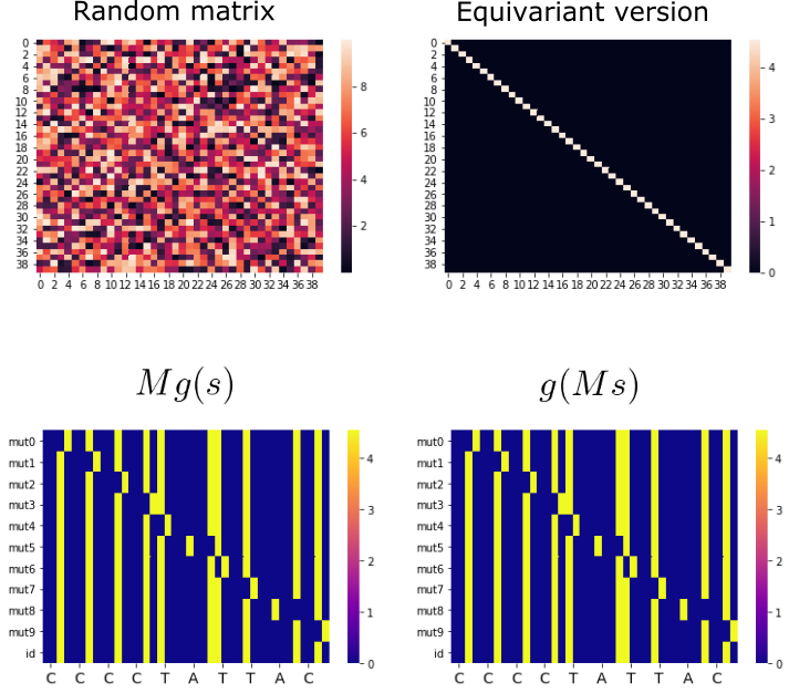
We can see it actually works ok with a random example:

Using the above method to get the equivariant version of a random matrix (first row). Second row: symmetry group actions showing that the resulting matrix does conform with equivariance constraints well.
Linear representations and equivariant basis
The problem with this approach is that it takes a long time. Each time we want to use the matrix of our module, we need to call get_equivariant_version to get the equivariant version which solves a possibly onerous optimization problem that can take up to 3 mins for each darn call. This is impractical even for our toy setting. To make this work, we have to make a couple of adjustments:
- Instead of using the arbitrary representations of $g(s)$, we’ll compute a linear approximation of the symmetry elements so that their actions over the sequences are $g(s) \sim \rho_g s$ for some matrix $\rho_g$. That is, our representation $\rho_g$ is the linear representation that we’ve mentioned above.
- Using the linear representations, we can see that any arbitrary matrix $M_{equiv}$ that satisfies \begin{equation*} M_{equiv}g(s) = g(M_{equiv}s) \sim M_{equiv}\rho_g s = \rho_g M_{equiv}s \end{equation*} should live in the null space defined by the linear equations \begin{equation*} (M_{equiv}\rho_g s M_{equiv}^{-1} - I) \rho_g = 0 \quad \forall s \forall g \end{equation*} We can get the basis of this space and its projection matrix $P$, and simply use it to project any arbitrary matrix $M$ into the space and get its equivariant version by just basic matrix multiplication, reducing the cost significantly. We call such basis the equivariant basis
Let’s code this up! Since these functions are attached to the symmetry in question, let’s make them methods of the class. First up, let’s “compile” linear representations for all of our generator functions. This is a straightforward least squares optimization problem:
class Sy
...
 def compile_linear_representations(self, Space, n_samples=100):
  def linear_rep_loss(mat, gen, samples):
     M_equiv = mat.reshape([Space.DIM, Space.DIM])
     return np.hstack(
         [
         np.dot(M_equiv, s.vec) - self.act(s, gen).vec
         for s in samples
         ]
     )

   samples = Space.sample(n_samples)
   self.vector_space = Space
   self.reprs = {}
   for g in tqdm(self.generators):
     x0 = np.eye(Space.DIM).ravel()
     res = least_squares(linear_rep_loss, x0, args=[g, samples], method='lm')
     self.reprs[g] = res.x.reshape([Space.DIM, Space.DIM])
   return self.reprs
Notice that compiling the representations “attaches” the vector space to the symmetry object. For our mutate symmetry object, we can compile its linear representations in a one-time, maybe expensive call:
mutate.compile_linear_representations(Sequence)
The resulting representations look like something this:

Examples of linear representations found by our equivariance basis projection method
Let’s briefly take a look at the compiled representations with more detail. Remember when I said that we implemented each mutation function in a weird way by cyclically shifting the vector with that np.roll call? Well, here’s the connection: you can clearly see that the representation for the mutation in the first nucleotide is basically the identity except for that square in the middle that contains a matrix like this:
\begin{pmatrix}
0 & 0 &0 &1 \newline
1 & 0 &0 &0 \newline
0 &1 &0 &0 \newline
0 &0 &1 &0 \newline
\end{pmatrix}
Which exactly corresponds to the cyclical shift operator! This was just for demonstration purposes – our mutation function need not be a cyclical shift, but could have been a mutation from any nucleotide to any other nucleotide, and its linear representation would just correspond to some permutation matrix. While we could have written the linear representations ourselves, I think it’s interesting and convenient that we can just think of our symmetry elements and their actions in terms of functions and let the computer find the appropriate representations.
Now that we have the linear representations for each generator of our symmetry computed, we can use them to compute the equivariant basis. Recall that given an arbitrary matrix $M$ we want a $M_{equiv}$ that satisfies
\begin{equation*} M_{equiv}g(s) = g(M_{equiv}s) \sim M_{equiv}\rho_g s = \rho_g M_{equiv}s$ \end{equation*}
and therefore that lives in the null space of the linear equations
\begin{equation*} (M_{equiv}\rho_g s M_{equiv}^{-1} - I) \rho = 0 \quad \forall s \forall g \in G \end{equation*}
This way of writing the set of linear equations is a bit cumbersome especially for a computer to solve. Luckily there’s this useful identity that says that if you have a system $AX = B$ with an unknown matrix $X$ then you can turn it into a standard linear system using Kronecker products $((B^{-1})^T \otimes A - I)vec(X) = 0$ where $vec$ is the function that flattens a matrix into a vector. We can then write out the linear system to compute the equivariant basis as a method in our Sy class:
from scipy.linalg import null_space

Class Sy:
 ...
 def compute_equivariant_basis(self):
   assert hasattr(self, 'vector_space'), 'Symmetry should have a vector space attached (via compile_linear_representations)'
   dim = self.vector_space.DIM
   lr = len(self.reprs)
   A = np.vstack(
       [
         (np.kron(np.linalg.inv(r).T, r) - np.eye(dim**2))
         for r in self.reprs.values() # matrix for each symmetry generator
       ]
   )

   Q = null_space(A)
   #Projection matrix:
   P = np.dot(np.dot(Q, np.linalg.inv(np.dot(Q.T, Q))), Q.T)
   self.Q, self.P = Q, P
   return Q, P
Notice how we are stacking each linear system for each generator representation matrix into a big linear system. Computing the equivariant version of any matrix then becomes super easy:
class Sy:
  ...
  def equivariant_version(self, R):
   assert hasattr(self, 'P'), 'Please first precompute equivariant basis (via compute_equivariant_basis)'
   return np.dot(self.P, R.ravel()).reshape(self.vector_space.DIM, self.vector_space.DIM)
Let’s try it out on a random matrix:
mutate.compute_equivariant_basis() # takes ~3 mins
R = np.random.rand(Sequence.DIM, Sequence.DIM) * 10
R_equiv = mutate.equivariant_version(R)
A random matrix and its equivariant version as found by our equivariant basis projection. The equivariant version is a very simple identity-like matrix that does conform to equivariance constraints (second row)
The equivariant version of the random matrix is indeed equivariant, but notice that it’s basically just the identity scaled by some scalar. This limits expressivity by a lot and it’s something that we will have to correct when implementing our equivariant module below.
Also note that while computing the equivariant basis still takes a while even for a toy example like this, it needs to be done only once. To scale it further to real examples we would need to make finding that null space more efficient, something that is a highlight in the linear MLP equivariant paper.
Putting it all together in an equivariant module
We have all the ingredients, let’s mix them into making an equivariant module!
import torch.nn as nn
import torch

class EquivariantLinear(nn.Module):
 def __init__(self, symmetry):
   super(EquivariantLinear, self).__init__()
   dim = symmetry.vector_space.DIM
   self.symmetry = symmetry
   self.W = nn.Parameter(torch.empty(dim, dim))
   nn.init.eye_(self.W)
   self.bl = nn.Bilinear(dim, dim, dim)
  def forward(self, x):
   W_equiv = torch.from_numpy(
                self.symmetry.equivariant_version(
                  self.W.detach().numpy()
                )
             ).float()
   xe = torch.matmul(x, W_equiv)
   return self.bl(xe, x)
Notice we have a bilinear layer that combines the equivariant transformed with the original input. This is necessary because of the lack of expressive power of the equivariant version (for our particular symmetry, it ends up being just the identity matrix scaled, which is not a very learnable parameter structure). We can then use this module to build any neural net, like this simple network that can be initialized to be made equivariant:
class SimpleNet(nn.Module):
 def __init__(self, equivariant=False):
   super().__init__()
   if equivariant:
     self.l1 = EquivariantLinear(mutate)
     self.l2 = EquivariantLinear(mutate)
     self.l3 = nn.Linear(Sequence.DIM, 1)
   else:
     self.l1 = nn.Linear(Sequence.DIM, Sequence.DIM)
     self.l2 = nn.Linear(Sequence.DIM, Sequence.DIM)
     self.l3 = nn.Linear(Sequence.DIM, 1)

 def forward(self, x):
   s = nn.SiLU()
   x = self.l1(x.type(torch.FloatTensor))
   x = self.l2(s(x))
   x = self.l3(s(x))
   return x.ravel()
A toy example: the TATAbox detector
Say we want to use our simple network with or without equivariance constraints to compute the binding energy of a TATAbox sequence motif, that can be perturbed by some mutations, to its transcription factor. We can build a simulated dataset starting from the TATAbox motif and perturbing it according to our mutation scheme:
from torch.utils.data import Dataset, DataLoader

MUTATE_MAP = {NUCLEOTIDES[i]: NUCLEOTIDES[i+1] if i < len(NUCLEOTIDES) - 1 else NUCLEOTIDES[0] for i in range(len(NUCLEOTIDES))}

def rand_seq(size):
 return ''.join(np.random.choice(list(NUCLEOTIDES), size=size, replace=True))

def perturb(seq, n_perturbs):
 perturbed_seq = seq
 for idx in np.random.choice(range(len(seq)), size=n_perturbs, replace=False):
   perturbed_seq = perturbed_seq[:idx] + MUTATE_MAP[perturbed_seq[idx]] + perturbed_seq[idx+1:]
 return perturbed_seq

class TATABoxDataset(Dataset):
   def __init__(self, size, max_perturbs):
     motif = 'TTATATATAT'
     self.sequences = []
     self.targets = []
     for _ in range(size):
       n_perturbs = np.random.randint(0, max_perturbs) if max_perturbs > 0 else 0
       seq = perturb(motif, n_perturbs)
       self.sequences.append(Sequence.from_str(seq))
       self.targets.append(np.exp(-n_perturbs)) # our “binding energy

   def __len__(self):
     return len(self.sequences)

   def __getitem__(self, idx):
     return self.sequences[idx].vec, self.targets[idx]
We can generate training and test sets with different numbers of perturbations and of different sizes and see how well a SimpleNet does with and without equivariance constraints. After scanning these 3 different testing parameters, this is what we get:
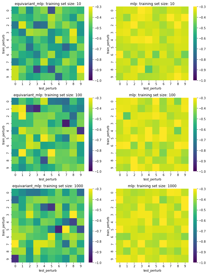
Test set loss of our simple network with equivariant versions (first column) and vanilla linear layers (second column) under several train/test mutation schemes (within grid) and training set sizes (rows). Darker (lower) is better.
The equivariant network does do a little bit better than the vanilla linear MLP but I was surprised that there wasn’t any pattern depending on the number of train/test perturbations. The sample size effect also doesn’t seem to be that great. Overall, equivariance does seem to be doing something to make the predictions better, though not dramatically.
Take home points
It’s fun and challenging to think about the symmetries that govern a particular problem, as it makes you think hard about the structure of the data and task at hand. It also expands the types of objects you can do machine learning on: in this toy example, our sequence of nucleotides were not just sequences of strings, but had an underlying mutation model – in the end they felt more like true biological sequences. It’s also interesting to note that with the proper API and abstractions, we don’t have to worry about group elements and representations, but rather think of them as functions (the group actions themselves) which I think is a more natural view, at least programmatically. The framework itself can be pretty powerful if only by putting us in the right state of mind to understand the data and task better. That said, I noticed there was some brittleness in symmetries. Sometimes our symmetry constraints are not clear cut but rather more fuzzy. For example, the mutation model we assume here is very far from reality. We would rather have a mutation model with transition probabilities between nucleotides. Such fuzzy symmetries are arguably more prevalent than rigid symmetries like rototranslational symmetries that govern some physical systems. We can perhaps deal with this by introducing some sort of probabilistic equivariance constraints, something that is hinted at in some recent work including the geometric deep learning book. Another disadvantage that I noticed is that equivariance (especially linear equivariance) comes at a cost of expressivity. Here, like in the equivariant MLP paper, we had to add a bilinear layer to boost the expressive power of our equivariant networks. Further, we used SiLU gates which are gated non-linearities that guarantee preservation of equivariant constraints. When you swap the SiLUs for ReLUs the vanilla MLP is basically as good as the equivariant version. All in all, I think the field is very promising and accelerating fast, but it’s still in an infancy of sorts, with lots of interesting and exciting stuff to figure out! I hope this post served to illustrate the concepts with a somewhat practical example, and don’t forget that all of the code is available in the colab notebook