Whenever I start thinking about a dataset that I need to model or start reading on a new field, one of the first things I try to get a sense of is the level of mechanistic understanding that we currently have on the phenomena that generated the data, and how that mechanism relates (generalizes) to other phenomena. One can usually get a sense of this by carefully looking at how folks are modeling simdata in the field. When performing such surveys, in my experience, there are two main types of models that come up. The first type corresponds to ‘descriptive’ models, which model the data at hand by focusing on its underlying shape, without making assumptions of how the parameters used to capture that shape interact. The second type corresponds to ‘mechanistic’ models, more ambitious models that state that the data arises from mechanistic interactions between its parameters. Importantly, the parameters could correspond to actual, measurable physical entities or abstract mechanisms that replicate in other datasets. Descriptive models focus on the data itself, almost in isolation, whereas mechanistic models are more bigger picture, where the data are only a means to an end of understanding a particular phenomenon. As such, they possess different predictive power: descriptive models make limited and typically qualitative predictions that rarely generalize outside of the distribution of the observed data. In contrast, mechanistic models try to generalize out-of-distribution scenarios and their predictions tend to be non-trivial (and easier to falsify). Similarly, the strategies used to refine and enhance each type of models (e.g. more samples, measure hidden variables, etc.) are different. Note that these model types are orthogonal to the generative vs discriminative classification, although mechanistic models tend to be generative since the generative frame of mind is compatible with finding hidden mechanisms that explain your data. This descriptive/mechanistic divide is very apparent in the nascent field of single-cell genomics and a certain type of measurements that have become all the rage in the field are a perfect example to explore the difference between the two types of models.

What is single-cell genomics and why should you care?

The pages of my first systems biology book were all about gene expression kinetics in single cells. The book focused on the statistical and computational techniques used to study the temporal patterns of gene expression of small gene networks like the lac operon and pals. The measurements to model were mainly readouts of a few gene products through time enabled by laborious microscopy protocols. Arguably, such high resolution measurements provide the most complete depiction of the system and if scaled genome-wide would come close to being a comprehensive portrait of the cell. After a decade since I bought that book, this vision has sort of come to fruition. Thanks to advances in cell isolation and sequencing, we are now able to measure the full transcriptome of thousands (and sometimes millions!) of cells at a scale. The price to do so is pretty low as well – both open source/maker movements and private companies have helped commoditize these measurements.

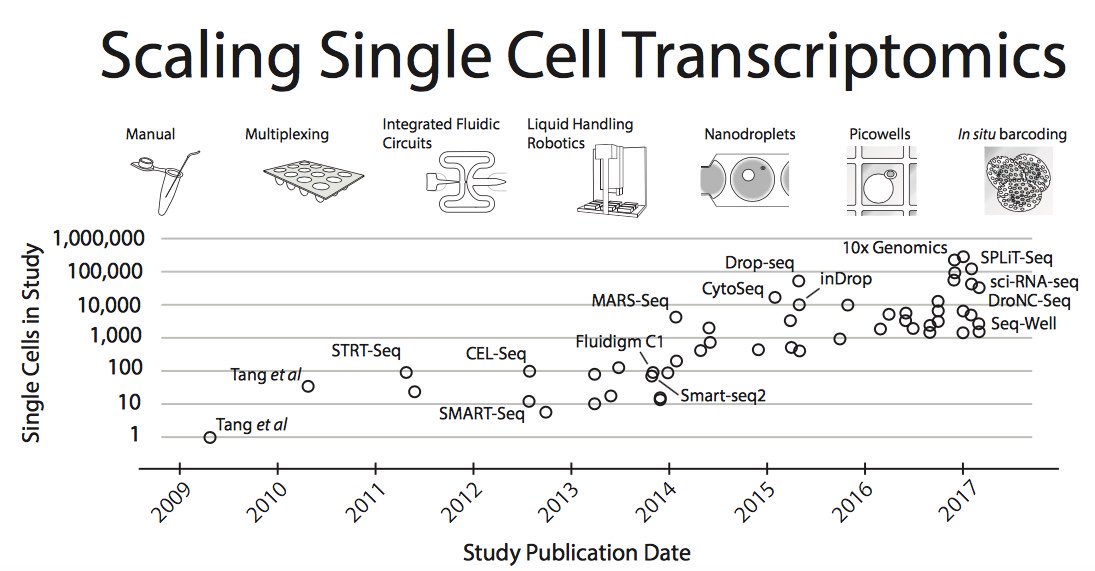Moore’s law in single-cell measurements. Taken from Svensson, et al. arXiv 2017

There is one catch though: the measurements are destructive and kill the cell. Unlike microscopy protocols, we’re not yet able to follow the evolution of the full genome as it’s expressed through time. Nonetheless, the ability to easily measure gene expression at single-cell level has taken the genomics world by storm. We are now well aware of our limited understanding of the repertoire (and even the very concept of) cell type in many organs and organisms. For instance, how do you define a neuron? Only through morphological characteristics? What if two neurons looked the same but were expressing different genes and had different behavior under similar conditions? Are they different cell types? How many actual cell types are there in the brain and how do they interact with each other? In the past few years, study after study have found that the gene expression configurations of single cells are complex, heterogeneous, and do not conform to a one-to-one mapping to our known cell types. The acceleration of accruement of these data has been so great that two luminaries of the field, Aviv Regev and Sarah Teichman, have sent out a call to arms to catalogue all human cells across time and space – the Human Cell Atlas – that promises to be as important as the human genome project. For once we have a map of all human cell types – once we know how cells flow from one type to another – we can may be able to achieve feats such as converting between seemingly unrelated cell types without too much effort (the holy grail of regenerative medicine), or pinpointing and avoiding drivers of potentially cancerous cell states, or simply understanding at a much more detailed level how organs function. Ideally, to best achieve these goals, we would want to get mechanistic models from this huge resource.

Cell trajectories: a non-linear rollercoaster

As mentioned above, one way of recording the molecular behavior of cells is by measuring the expression of a handful of genes through time, yielding multivariate cell trajectories of gene expression. Complex cell processes such as infection response, quorum sensing, and metabolic regulation have been dissected in detail through these measurements. Not only do these measurements link gene expression to higher order phenotypes, but they reveal dependencies between genes, essentially probing the gene network that underlies the phenotype directly. The models arising from fitting these data come in the form of stochastic processes that describe the kinetics of the system, usually through some master equation – a prime example of a mechanistic model. Although the process rules of the gene network could themselves be simple, the resulting behavior is highly non-linear, with potential bifurcations, attractor states, and cycles that bestow upon the cell a wide range of tunable complex behaviors. Many times, the molecule count in these stochastic processes is low, which amplifies the noise in the system, adding yet another element to its complexity. This intrinsic noise plays a critical role in the cell’s fitness landscape and either has to be controlled or can be harnessed to modulate behavior (the wikipedia page is actually pretty informative if you want to know more on this topic).

Unfortunately, in the vast majority of cases we cannot study a cell’s behavior in such detail, most of the time due to experimental intractability of the system. Furthermore, if we want to probe the expression of more than just a few genes, the cheap and scalable sequencing techniques mentioned in the previous section that we could use to do so require cell lysis. Nevertheless, even through these more coarse-grain, asynchronous measurements we can make out gene expression manifolds that are a static, snapshot representation of the actual cell trajectories. Sure, we’re not able to see the evolution of the system directly, but by capturing the intermediate cell states and interpolating smartly, we could get a notion of the overall shape of the process. This became apparent in several studies in 2014 and generated a lot of excitement – we were finally able to catch a higher-resolution glimpse of previously inaccessible developmental processes such as cell type differentiation and cell fate decisions. A deluge of methods for ‘trajectory inference’ from these static measurements that used everything from Gaussian processes to simple nearest-neighbor graphs followed (seriously, everyone and their mother in the field have made one version of a trajectory inference algorithm, myself included). All of these models are firmly in the descriptive realm: they cannot directly model the temporal gene expression patterns, but they can describe cell states that appear to be interconnected. As with any descriptive models, the predictive power they hold is tied to how effectively they summarize the data so we can visualize it and how they avoid potential confounders in fitting the data’s distribution (e.g. getting the manifold shape right by not connecting two nearby but unrelated states, like connecting points in two different turns of a swiss roll). In contrast to the mechanistic models of temporal gene expression trajectories, their predictions are mainly qualitative: the importance of a gene may or may not be related to how its expression changes from one part of the trajectory to another.

But, how can we get from these descriptive models to more mechanistic ones? What, if any, additional experimental capability we need to start dissecting cell trajectories in detail at a genome-wide level? Below, I’ll try to explore these questions using a simple gene expression trajectory system.

The Lorenzian cell

Consider a toy example of a gene expression trajectory. Suppose that we have a cell with three genes whose evolution of gene expression can be written as the following dynamical system:

\begin{cases} \dot{g_1}(t) & = 10(g_2(t) - g_1(t)) \newline \dot{g_2}(t) & = 40g_1(t) - g_2(t) - g_1(t)g_3(t) \newline \dot{g_3}(t) & = g_1(t)g_2(t) - 3g_3(t) \newline \end{cases}

This is the well-known Lorenz system. For simplification purposes, we won’t add intrinsic noise to the equations (i.e. they’ll be deterministic) and we will be working in log-space to allow gene expression, which is always non-negative, to take on negative values. Finally, we assume that g2 is an unknown gene that we’re not quantifying (e.g. some transcribed repetitive element in the genome). This is what our trajectory looks like:

Our toy system

Now, suppose we measure this system by sequencing a population of cells all undergoing this trajectory asynchronously using (a very low-throughput) single-cell RNA-seq assay that measures only genes g1 and g2. Say we only have money left in the grant to measure 20 cells, our data points would then look somewhat like this:

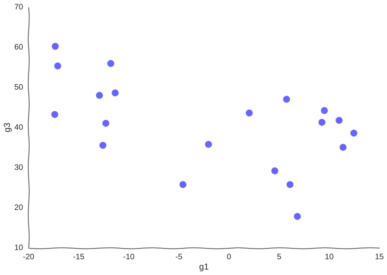Too few samples

Note how much of the information in the original system is destroyed – we can only conclude that there are two cell populations that may or may not be part of the same trajectory – there is no glimpse into mechanism, we just know of two blobs of data points. Let’s try increasing the information.

With apologies to Randall Munroe

More samples

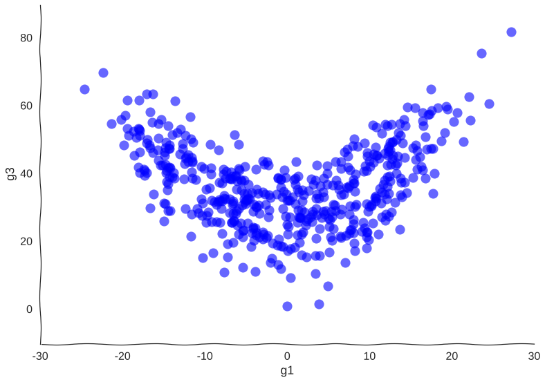
Suppose we get lucky in the next grant round and we get money to sequence a whole lot of cells. We unfreeze some samples and sequence 2000 more cells. After doing hair-pulling batch correction to combine the datasets (the confounders in single-cell measurements can get pretty scary), we end up with this data:

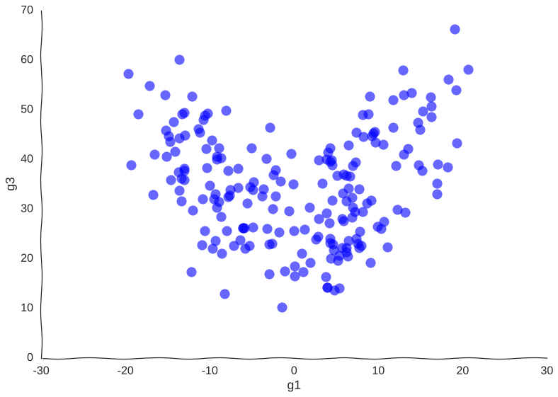A bit better

And here’s a kernel density estimation of the distribution:

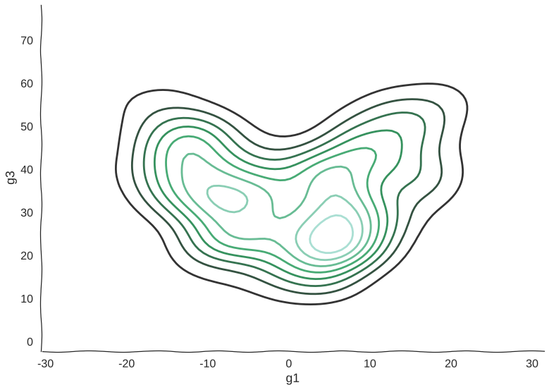Scatterplots can be misleading sometimes

Now, we can see clearly the structure of the trajectory’s manifold. We can even compute a principal curve, a smooth curve that follows the local mean of the data, for a crude approximation of the trajectory. In essence, this is what all trajectory inference methods do:

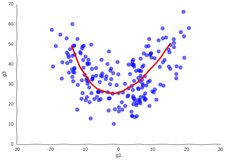Why so serious?

We get the overall trend from one attractor to another and we can now confidently say that genes g1 and g3 are correlated somehow. However, many mechanistic details are lost. For example, we wouldn’t be sure if the trajectory is cyclical or if the cell goes from one place to another, never to return. No matter how many more measurements we make, the result will be the same.

Organelles not to scale

Measuring a known unknown: time

Suppose we somehow get the awesome power to sequence time itself and we are able to barcode our static samples with the exact timepoint in the trajectory from whence they came. We would be able to color this readout and for starters observe that cells do indeed revisit regions of the manifold.

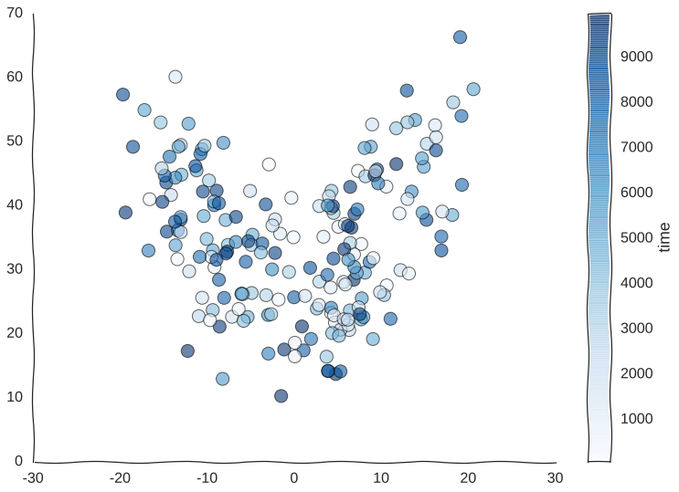Still kind of a mess

But what model can we use to fit these data? We could, for example, thread a two-dimensional Gaussian process through our cells.

With apologies to Jackson Pollock

As expected, due to how the samples are randomly interspersed, we get a noisy fit, but the general trend of back-and-forth of the trajectory is captured. While we get a bit closer to modeling the behavior of the cell, we still don’t quite yet have a mechanism for it. Arguably, the kernel choice for the Gaussian process (in this case, a Matern kernel), can yield some insights into these mechanisms, but parsing out the actual dependencies between variables would be non-trivial and qualitative.

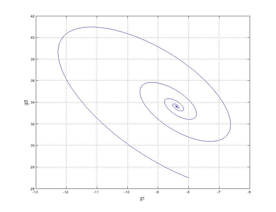
Can we fit a more mechanistic model to it? We could try to model the system by guessing a functional form for an ordinary differential equation (ODE) model that fits the data, something called non-linear system identification. I found an interesting paper that takes this route by performing sparse symbolic regression to obtain an ODE that describes the data. However, when fitting to genes g1 and g3, we run into trouble (plot style changes since this is in matlab)

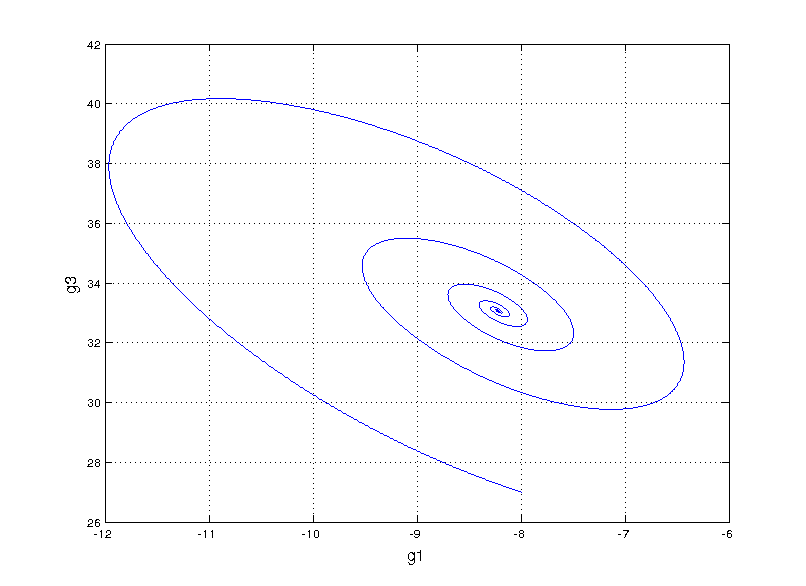Not even close

This is totally off the mark! Even exploring our vocabulary of functions for the symbolic regression by adding high order polynomials (up to 5) and sines and cosines we still get something that’s hilariously wrong. Here, we start getting a hint that something fundamental is missing.

I spent way too much time drawing this with a mouse

Controlling the sampling distribution

Maybe our measurements are just sampled too at random, which can break local information. Suppose we can capture cells at regular intervals instead of sampling uniformly at random. This regularity is not really all that apparent when we plot the raw data.

Still smiling

However, it is very helpful to our Gaussian process. When we re-fit the data to it, we get a pretty good picture of the system’s behavior:

I was kind of surprised this worked with little tweaking

If we would wish to continue to travel the Gaussian process route and make it as predictive as possible (for example, forecasting future possible events of the system), we would need to rethink on how to partition the data to generalize the periodicity and offset of the attractors. Looking around, I actually found a paper that does precisely this.

But we want to be done with descriptive modeling! Let’s fit our sparse ODE system to the regularly sampled data:

Not even wrong

Same horrible result! This confirms that something is amiss, something we’re not measuring…

Wonder why I drew a eukaryote cell

Measuring an unknown unknown

Using an ODE of just two variables, you’d be hard pressed to find a system with a twin-attractor behavior (I’m no dynamical systems expert – is it even possible?). So in trying and failing to fit our mechanistic model, we might hypothesize that there’s an extra variable. Recall that we were oblivious to the fact that g2 existed since we couldn’t measure it with our short read technology. Switching to nanopore sequencing, say we are now able to capture g2. Let’s try our symbolic regression ODE once again!

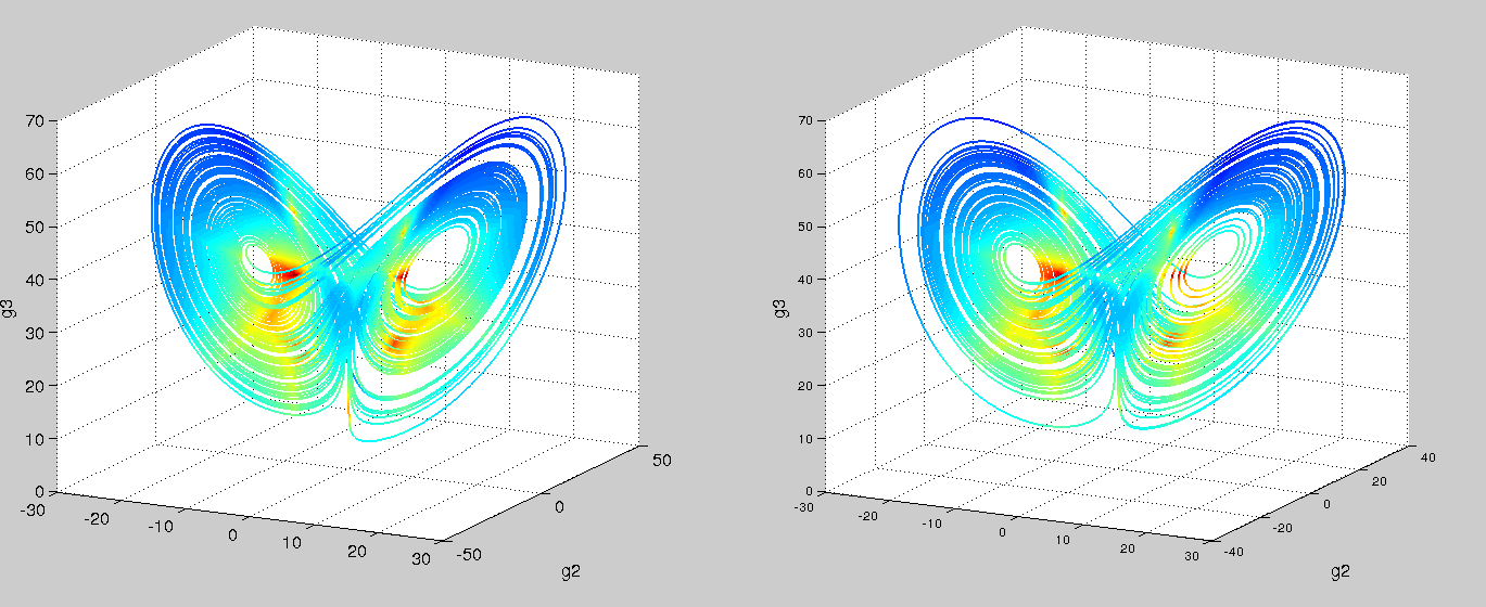Left is real data, right is predicted. Colored by timestep. Using the code from Brunton, et al. PNAS, 2016

Success! And with just polynomials (at most degree 3) too. A more comprehensive search space would probably yield the linear-plus-interaction-terms form of the actual Lorenz system. We can then go and test these models with follow-up, detailed kinetic measurements.

From 3 genes to 30K+

This was a hypothetical study of a toy system of three genes, but consider that state of the art single-cell measurements probe more than 30000 different transcripts (the majority of the transcripts are not expressed in a given cell, but even ones that are expressed tend to be in the hundreds to thousands). Sure, getting to the point where we can sample trajectories at the level of detail of the final steps of this blog post would require revolutionary experimental advances – but it doesn’t seem at all unfeasible. In the not so distant future the day will come when we can get such data. Imagine then the complex behaviour of such a high-dimensional dynamical, stochastic system. The vast space of gene networks that could explain the data would be folds upon folds of magnitude more than the particles in the universe. Fitting a toy system like we did in this post is akin to climbing a small hill in a park, while the Himalayas loom in the distance. Maybe we should stick with descriptive modeling for now.

A steep road ahead

Back to posts