I first found out about probabilistic programming in my later years of grad school when, looking for good tutorial on Bayesian inference, I stumbled upon the excellent Bayesian Methods for Hackers, which heavily features PyMC. I was (and in many ways I still am) a neophyte Bayesian methods, having ignored the quasi-religious sermons that my friends in operations research and actuarial sciences gave to any passer by, swearing by the name of simulation with strange and arcane words ending in UGS and AGS. It was the concrete simplicity of a PyMC model that caught my eye. I was trying to do maximum a posteriori fit to a statistical model and here I was trying to calculate gradients by hand (this was before autodiff methods caught on), putting in ridiculous constants to avoid gradient descent to go into lala land and having generally no idea how to include all the constraints that I wanted. AFter reading the PyMC tutorials, I wrote the same problem as a PyMC model – it was barely 20 lines of clear and concise code. I was thrilled! But then I pushed the inference button and got a whole spew of samples. I started learning about burn ins and thinnings, autocorrelation and adaptive methods (this was also a time where Hamiltonian Monte Carlo had not quite yet reached mainstream implementations), and how in general it was impossible to tell for some degree of certainty if whatever sampling you were doing was correct. It was also somewhat slow due to the number of variables in the model. I ended up abandoning my PyMC implementation in favor of another one that (ab)used the Levenberg-Marquardt method to sort of solve the problem. But the core idea behind PyMC and probabilistic programming got stuck in the back of my mind. Ever since, I’ve been following the evolution of PPLs and many times returned to try them. Sometimes they work pretty well and the recent implementations that take advantage of Hamiltonian MC and GPUs make the sampling really fast. There’s also a whole gamut of tests like divergence diagnostics that make it easier to see if your sampling is going awry. These advances are great, but it’s still a pretty big project to satisfactorily explore and fit a medium to large statistical model – there are prior predictive checks, there’s the complexity of the sampling itself, and making sure you got it right. For some problems, especially ones where it’s critical to get a detailed and solid answer, such checks and challenges are a boon as they do not allow you to make progress unless you make sure everything is in order. It also works very well and out-of-the-box for simple, low-dimensional (as in one or two parameter) models. For the majority of problems in between those two extreme cases, however, I’ve found it difficult to justify the rabbit hole that Bayesian inference can be. Or I don’t know, maybe I’m just lazy. In part to try to address this void and in part to learn more about the core ideas behind the implementation of probabilistic programming languages, I set out to try and implement my own.

To be clear, I’m not sure the world needs yet another vanilla probabilistic programming language, and I’m certainly not the person to carry this the state of the art forward. I think the current ones in production like Stan, PyMC, or [num]pyro are already pretty great and the ones in serious development have lots of exciting ideas to explore and contribute (I’m particularly excited by mcx which has an inference-first philosophy and promises to do simple graphical manipulations like do operations really simple). However, there are also some ideas that I’ve been meaning to explore for a while and implementing them in a PPL might trigger some conversations around them. To set the controversial spice level to the max, I tried breaking some Bayesian taboos in the process. To start, I laid down the list of things that bugged me about PPLs and Bayesian inference in general:

1. Requires too much knowledge about inference: I don’t want to learn the intricacies of differential geometry to understand what the inference method is spitting
2. Requires too much knowledge about distributions: Ideally, I don’t want to have to learn stats to use this either, especially what distribution is suited for what data because of its tails or whatever
3. Takes too long to sample a model (and iterate over it): Especially for “deep” hierarchical models, or models with too many variables
4. Takes too much effort to know if you’re right: All those divergence diagnostics are great, but they are still confusing to non-Bayes geeks.

While the generally correct answer to the above is simply “don’t be lazy and actually learn to model!”, I believe there’s also opportunity for building a framework around a limited combination of models that are most user agnostic. Sort of like some curve fitters and optimizers where the user is not expected to know if Newton-Raphson is or isn’t a forgotten youtuber. In any case, based on the list of things that bugged me about PPLs, I set another list of ground rules for my PPL implementation that sort of tries to address these issues:

1. No sampling, only use full enumeration/exhaustive methods: Your sampling can’t be wrong if you don’t sample!
2. No obtuse distribution names: What’s normal about a Normal distribution anyway?
3. Don’t use the computational graph framework du jour: It changes with the season. Do you remember how to use theano? What’s theano? Yeah my point exactly.

I also came up with a cute name for it: simppl. So with just that in mind, and without reading basically anything on how to implement a PPL, I set off…which was a mistake.

Models as programs, samples as executions

Right from the beginning it was clear that I would need to “design” my way out of using sampling and standard distributions. So I tried thinking on how a user might want to use the PPL embedded within already established data structures like dataframes. In short, I put together the API first, whipping up some simple distributions and some fancy pandas integrations, thinking that later on I would build the core inference engine that would make it just work. I mean, a PPL is basically just Bayesian inference with some syntax sugar on top right? WRONG The code I ended up with was messy and made some very questionable twists and turns to adapt to my way of thinking. At one point I just decided to discard it all and actually read how other people have tackled this. The best guide I found to this end was DIPPL, which uses WebPPL as a language to teach how to make PPLs (I eventually found out about an excellent paper introducing probabilistic programming language design from one of Rémi Louf’s tweets, which goes even deeper into the topic). The main idea is that a program that includes random computation as some of its steps is a probabilistic model for which each execution is a sample of it. Additionally, you have to have a way to score each execution which both depends on the likelihood assigned to each random variable in the model and any additional information like observations. So in essence, inference becomes a control flow problem, you just have to find a way of saving the model as some future computation, execute it under different values (samples) and score them. This is both a lot less code and a lot more intuitive.

A quick computational graph implementation

On my second attempt, I decided to follow the “models as programs, inference as control flow” mantra. WebPPL achieves this using a very elegant application of continuation passing style. Continuations are a control flow structure from the functional programming world where you can store a computation sort of as a template and apply it in different contexts (e.g. storing the “skeleton” of the model and then replacing each distribution with a given value during each execution). Continuation passing style transforms any function into another function that uses passes continuations as “contexts” for each execution. If there’s anything like poetry in computer science, it’s continuations. Except that I’m no poet, nor a functional programmer. I was trained under the boot of object orientation, writing enterprise java beans and kneeling before JBOSS (if you know what any of this means then congrats, you’re old like me). So what’s the horrible stateful sibling of continuation passing style? That would be a computation graph, at least for this application. So I made a dead simple one comprised of one abstract base class, CNode, and three other classes Constant, Variable, and Op, which represent exactly what you imagine: constants, variables, and operations between them. These classes are orchestrated by a ComputationRegistry class, which is instantiated as a singleton in a COMPUTATIONAL_REGISTRY instance. It’s a rather naive and unremarkable computational graph implementation, but it does have one interesting hack as illustrated by the Variable constructor that calls the ComputationalRegistry.call_or_create_variable:

class Variable(CNode):
    def __new__(cls, name: str, *args, register: bool = True, **kwargs) -> Any:
        return COMPUTATION_REGISTRY.call_or_create_variable(name, cls, register, *args, **kwargs)

class ComputationRegistry:
        ...
        def call_or_create_variable(self, name: str, cls: Type['Variable'], register: bool, *args, **kwargs) -> Any:
            # If the variable is not yet registered, create it and return it....
            if name not in self.current_variables or not register:
                instance = super(Variable, cls).__new__(cls)
                instance.name = name
                instance.__init__(name=name, *args, **kwargs)

                if register:
                    self.variable_inits[name] = [args, kwargs]
                    self.current_variables[name] = instance
                return instance
            # ... or if we are actually unrolling the computation,
            # swap the variable with the values in the definitions
            if len(self.current_definitions) > 0:
                return self.current_variables[name].call(self.current_definitions)
        ...

Class instantiation in python first goes through __new__ and then is initialized via __init__. We can take advantage of this by letting the COMPUTATION_REGISTRY decide if a new variable needs to be created and registered; or if it already exists in the computation graph and the computation is currently being unrolled, then swap the return value with the current definition of the variable. This allows us to sidestep needing to parse code that involves computation graph variables: we can simply call a variable once to register it, then swap it with different values on each subsequent execution. After the computation graph implementation, distributions are just Variables with some additional methods, like a log-likelihood. At the end this second attempt of implementation, however, I realized that you could do away with the computation graph entirely, with some caveats, but decided to put off yet another rewrite for a future version.

Exhaustive Inference

Remember, I said no sampling inference algorithms or anything that requires too much knowledge of probability. This means no MCMC, no variational inference, and I won’t be satisfied just doing maximum a posteriori. This only leaves exhaustive, or full enumeration inference; in which we score each and every possible execution allowed by the supports of the model’s distributions and normalize their weights to make them probabilities. The implications of this is that our distributions need to (1) have finite support (so discretized in some way) and (2) we can only have a finite set of variables in the model. Thus, simppl is what people call a first order probabilistic programming language or FOPPL, in which things like recursion and first order functions are node allowed.

A first simppl model

To illustrate how using this feels, let’s try a simple simppl model for a biased coinflip:

from simppl.distributions import Pick, Flip
from simppl.utils import capture_locals
from simppl.inference import Exhaustive

import numpy as np

# All observations are 2D arrays, rows are samples, features are columns
tosses = np.array([0, 0, 0, 1, 0, 0]).reshape(-1, 1)

def coinflip_model(tosses=tosses):
    p = Pick('flip_probas', items=[0.1, 0.5, 0.8, 0.9])
    coinflip = Flip('coinflip', p=p, observations=tosses)

    capture_locals() # --> capture_locals grabs the state of all variables
                     # above it and records , them at each execution..
                     # these values can then be inspected after inference...
    return coinflip


env = Exhaustive(coinflip_model)

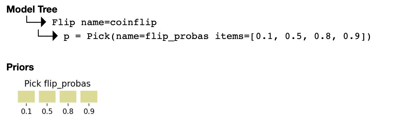
Hopefully this is somewhat self-explanatory. Pick and Flip are uniform and Bernoulli distributions respectively, inspired by how WebPPL calls them. The capture_locals utility function allows you to capture the “state of the world” at each point during the computation by recording all the variable values at that point. Notice how tosses is part of the function model’s parameter. This isn’t required as there is no limit for coinflip_model in terms of scope, but I find it to be clearer that way. What Exhaustive returns is a RandomComputationEnvironment which contains two main things: an executions dataframe with all of the executions, capture variables values, and their probability, and a model variable that has a structured version of the model. For this example, the executions dataframe looks like this:

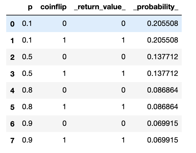
with which you can quickly inspect marginal posterior distributions:

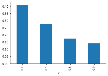
The model can be readily inspected in a jupyter notebook by just doing env.model in a cell:

The SomeValue distribution

Remember that I didn’t want to put in a laundry list of distributions with arcane names. Instead, I asked myself, to someone completely agnostic to probability distributions, what is the most basic API I could provide?. How do we deal with uncertainty in everyday conversation? What’s the equivalent of a random variable in natural language? I ended up gravitating towards the phrase “this quantity is some value between such and such, around these values, but mostly this value” as encapsulating the spirit of a random variable. Translating this to a distribution constructor it yields something of the kind SomeValue(between=[low, high], around=[these, values], mostly=this_value). I found this to be intuitive and even a bit SQL-ish. How then do we implement this into an actual distribution? At first I thought that a mixture of Gaussians with modes in the around clause and a less variance mode in the mostly value would do the trick, but I ended deciding to do something “peakier” where the probability mass radiated from the around values decaying linearly with some factor and from the mostly value decaying quadratically. This functional form just ended up making more sense visually to me, especially when discretizing (remember, we are only doing exhaustive inference, so we need finite and hopefully smallish support for each distribution), but this is really arbitrary. I also forewent adding a variance parameter, which might provoke swoons, but I just couldn’t find a satisfying natural language descriptor for it. Again, this is pretty arbitrary and I am happy to hear suggestions of how to otherwise implement the SomeValue distribution.

Fermi problems

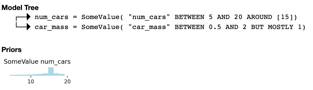
I’ve found that simppl fits nicely into the “Fermi problem” use case, where the solution is some back-of-the-envelope calculation with rather lax constraints. For example, say we want to answer the question “What is the mass of all the automobiles scrapped in North America this year?". A quick google search reveals that the number of cars scrapped in the US is around 15 million each year. I have an intuition that a car’s weight is some value between 0.5 to 2 tons. The model is straightforward:

from simppl.distributions import SomeValue

def scrapped_cars_model():
    num_cars_scrapped = SomeValue('num_cars', between=[5, 20], around=[15]) # in millions
    car_mass = SomeValue('car_mass', between=[0.5, 2], mostly=1) # in tons
    return num_cars_scrapped * car_mass * 1e6

There’s no inference to be performed here, but we can still take a look at the distributions. Let’s look at the underlying model:

Inference in a univariate model

How about something a little bit more complex? Let’s say we are trying to model the cytotoxicity of some compound of interest. We do this by spiking the compound at some concentration into the media of some cells in vitro and watch how their growth is stunted, typically called growth inhibition. We use a simple model where the log of the growth inhibition is a sigmoidal response on the concentration of the compound scaled by its toxicity. The toxicity value will be the one we will want to infer:

def sigmoid_response(toxicity, log_concentration):
    return 1 / (1 + np.exp(toxicity * log_concentration))

Let’s generate some toy data:

log_concentration = 1
true_toxicity = 0.6
inhibitions = (sigmoid_response(true_toxicity, log_concentration) + np.random.randn(2) * 0.001).reshape(-1, 1)

We can use the SomeValue distribution as both our likelihood for the data and our prior on the toxicity:

def cytotoxicity_model(inibitions=inhibitions):
    toxicity = SomeValue('toxicity', between=[0, 2], around=[0, 1.5], mostly=1.3)
    inhibition = SomeValue(
        'inibition',
        between=[0, 1],
        mostly=sigmoid_response(toxicity, log_concentration),
        observations=inhibitions
    )

    capture_locals()
    return inhibition

After inference, we can see how our model starts giving weight to the right toxicity:

Going multivariate: the SomeThing distribution

The model above deals with only one concentration, but of course we would want to measure the inhibition at different concentrations. We could in theory put a different SomeValue distribution for each concentration, but that would quickly explode our exhaustive inference as we encounter the curse of dimensionality. What’s needed is a multivariate analog of the SomeValue distribution. Here, things get really dicey: how do you discretize in multivariate space? There are no right answers to that question, so instead, what I decided is to let the user define a set of samples that would mostly represent the support of the distribution. We can then discretize the space defined by those samples by performing some clustering on them and choosing the medoids of each cluster as discretized representatives (I chose spectral clustering for this purpose but really any algorithm could do). We can also add a mostly parameter that skews the probabilities towards that region of the support by projecting to the nearest representative. The multivariate analog of the cytotoxicity model looks like this:

# We now have 5 concentrations
log_concentrations = np.array([-5, -3, -1, 1, 2])
true_toxicity = 0.6
n_obs = 2
inhibitions = (sigmoid_response(true_toxicity, log_concentrations) + np.random.randn(n_obs, 5) * 0.001)

# Sample inhibitions to define support for our SomeThing distribution
inhibition_space = np.random.uniform(
    low=sigmoid_response(0, log_concentrations),
    high=sigmoid_response(2, log_concentrations),
    size=(100, 5)
)

def cytotoxicity_model_mv(inibitions=inhibitions):
    toxicity = SomeValue('toxicity', between=[0, 2], around=[0, 1.5], mostly=1.3)
    # SomeThing is our "error/likelihood model"
    inhibition = SomeThing(
        f'inibition',
        samples=inhibition_space,
        resolution=80,
        mostly=sigmoid_response(toxicity, log_concentrations),
        observations=inhibitions
    )

    capture_locals()

# Inference
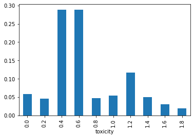
env = Exhaustive(cytotoxicity_model_mv)

# Plot posterior for toxicity
# round toxicities to second decimal for plotting
(env
 .executions
 .assign(toxicity=lambda df: np.round(df['toxicity'], 2))
 .groupby('toxicity')['_probability_']
 .sum()
 .plot.bar()
);

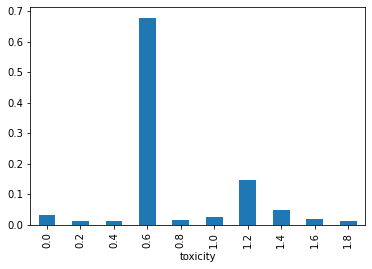
Sometimes we get a nice result like the above, but sometimes we don’t and it really depends on how we define and sample the inhibition_space which ends up deciding the support of the SomeThing distribution. I know what you’re thinking: “I thought you say no sampling!”. Yes, unfortunately this is a thinly veiled attempt to put the onus of finding the support of the distribution upstream, to the user. Typically, we would sample during inference in search of the “true” support, e.g. where the distributions take on a non-negligible probability. Here, I’m directly asking the user to provide this to keep simppl as simple as possible – the hard work of finding the support can never be avoided. An interesting side-effect of being asked for the support beforehand is that I ended up trying different ways of defining inhibition_space, but it was glaringly obvious when the support was the wrong choice as the posterior distribution on toxicity yielded very uniform-looking distributions.

One last example: molecule identification

While a bit disappointing because of the whole support definition issue, the SomeThing distribution does have a neat property: since it uses spectral clustering to discretize, which is a kernel method, you really only need a notion of similarity between your “things” to define the distribution. To illustrate, let’s say that we have a mystery solution which we know it’s some purified form of one of a list of molecules. What we can do to decipher which one of these molecules comprises the mystery solution is measure it in some way (e.g. take its UV spectrum) and compare the measurement with theoretical predictions of each of our candidate molecules. We’ll call this measurement the molecule’s observable and we assume we can simulate it from first principles given the molecular structure or composition in some way. To simplify things, in this example our observable will be a simple count of the number of carbons in the molecule (the measurement could be something that correlates with number of carbons, like boiling point). First, let’s assume we have the list of molecules as a list of SMILES strings. We can use RDKit to manipulate the molecules:

from rdkit import Chem
from rdkit import DataStructs
from rdkit.Chem.Fingerprints import FingerprintMols

# Assume that our molecules are a list of SMILES in the "smiles" variable
molecules = np.array([Chem.MolFromSmiles(x.strip()) for x in smiles]).reshape(-1, 1)

We can use the fact that we can measure similarity between molecules to aid our inference – to do so we use established methods in chemoinformatics using molecular fingerprints.

# Precompute molecular fingerprints for similarity
fingerprints = {m : FingerprintMols.FingerprintMol(m) for m in molecules.flatten()}

# Define a similarity function to be later used in our model
def molecule_similarity(mols1, mols2):
    sims = [
        DataStructs.FingerprintSimilarity(
            fingerprints[mol1],
            fingerprints[mol2],
            metric=DataStructs.TanimotoSimilarity
        )
        for mol1 in mols1.flatten()
        for mol2 in mols2.flatten()
    ]
    return np.array(sims)

Our observable will just count the carbons in our molecules and will return that number times some constant, just for kicks.

from simppl.utils import register_function

# We need to register the RDKit's GetSubstructMatches function to be able to use
# it in our computation graph
def count_carbons(mol):
    return len(mol.GetSubstructMatches(Chem.MolFromSmiles('C')))

# register_function attaches the function both to simppl's computation graph and
# to the class of our choice
register_function('count_carbons', count_carbons, cls=Chem.rdchem.Mol)


def simulate_observable(molecule, constant):
    return constant * molecule[0].count_carbons()

Note that the content of count_carbons doesn’t matter, it can even be a call outside python and it will still work. With these ingredients in place we can finally write out our model:

# Guess range for observable
o = np.array([simulate_observable(molecules[i, :], c) for i in range(molecules.shape[0]) for c in [0.5, 5]])
min_o, max_o = o.min(), o.max()

# Some toy observations
true_molecule = molecules[10, :]
true_constant = 2
n_obs = 2
toy_observables = (simulate_observable(true_molecule, true_constant) + np.random.randn(n_obs) * 0.01).reshape(-1, 1)

def molecule_observable_model(observables=toy_observables):
    # Note how we can use the molecules directly! We only need the molecule_similarity function
    molecule = SomeThing('molecule', samples=molecules, resolution=10, affinity=molecule_similarity)
    constant = SomeValue('constant', between=[0.5, 5], mostly=1)
    observable = SomeValue(
        'observable',
        between=[min_o, max_o],
        mostly=simulate_observable(molecule, constant),
        observations=observables
    )
    capture_locals()

# Inference
env = Exhaustive(molecule_observable_model)

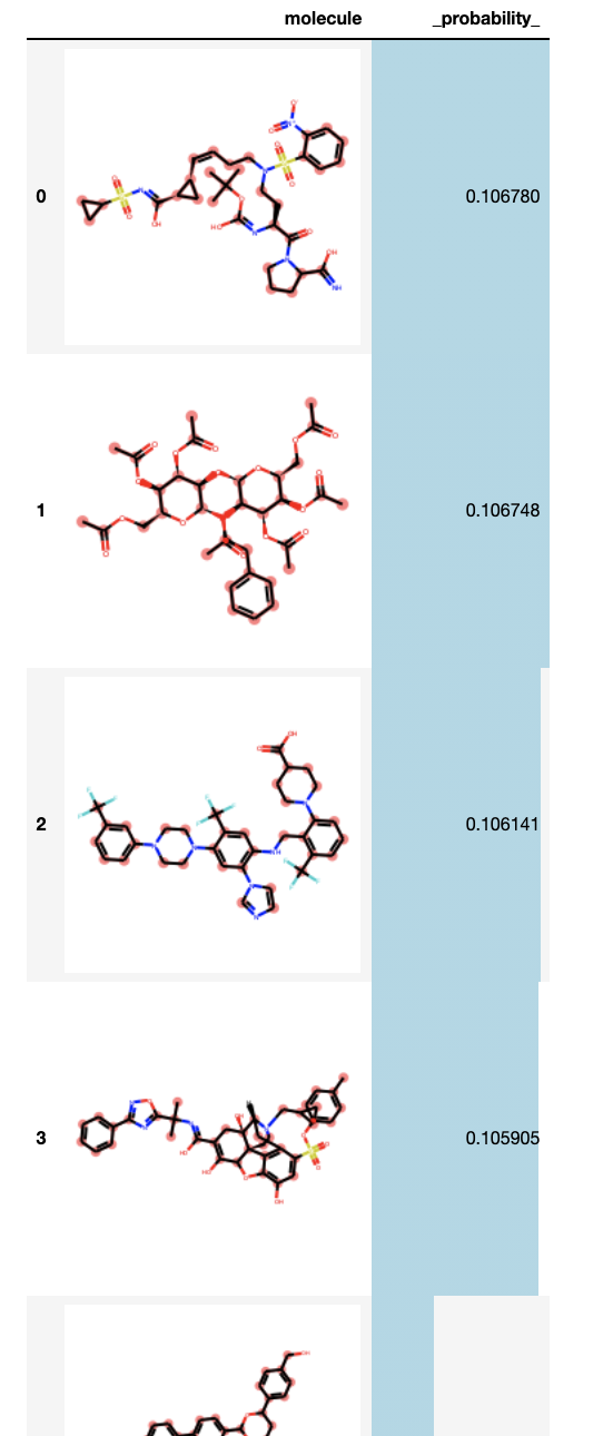
Let’s visualize the results, using RDKit’s helper pandas functions

from rdkit.Chem import PandasTools
from IPython.display import HTML

HTML(
    (env
     .executions
     .assign(
        molecule=lambda df: df['molecule'].apply(lambda x: x[0])
     )
     .groupby('molecule', sort=False,)['_probability_']
     .sum()
     .sort_values(ascending=False)
     .reset_index()
     .style.bar(subset=['_probability_'], color='lightblue')
     .render(escape=False)
    )
)

Conclusions

My simppl implementation of a PPL did fulfill one of its goals: I learned a ton doing it and appreciated the obstacles, limitations, and future promise of PPL with much more detail. It does not, however, quite fulfill my original goal of producing an “out-of-the-box-plug-and-play” solution to statistical modeling that anyone could use. I’m constantly reminded of Stephen Boyd’s definition of a “mature technology” (can’t find the quote, but it’s something he repeated often in his convex optimization class at Stanford): it’s mature when anyone without domain expertise can use it. Linear regression is a mature technology, as is the whole notion of least squares. General convex optimization is not quite there yet, but is getting pretty close. Bayesian inference however, is still further behind. I hope some of the ideas in simppl can start conversations toward maturing Bayesian inference with an eye of the end user rather than the mathematics behind it, I’m sure there’s a subset of it that can be packaged in a right way to make it available to anyone. You can take a look at simppl’s repo . All of the code in the post is summarized in a notebook there.

Coda: alternative unorthodox paths to PPLs

Before settling on the current version of simppl, I thought of taking other contrarian paths towards my implementation:

Qualitative probability: There’s a whole very academic field dealing with qualitative probability, where instead of assigning a probability quantity to an event, we only know if one event is more probable than others, inducing an order of what’s more probable to happen. The result is a system that’s embedded within the mathematics of logic rather than algebras. While intriguing, I found it hard to work with past very simple examples, and there’s very sparse literature on this so I ended up abandoning the idea.

Natural language descriptors as probabilities: What if instead of assigning probability quantities in our model we simply say that an event is “likely” or “improbable” or something more akin to a natural language descriptor. The CIA has actually studies how these uncertainty statements map to actual probabilities in our mind. At first I thought that this could be used to reduce computational cost in inference, but unfortunately it doesn’t help all that much.

Back to posts